U‑Net vs Vision Transformers for Land Cover Change Detection

Land cover change detection sits at the intersection of machine learning, geospatial computing, and environmental science. The technical task sounds simple: compare imagery from two dates and identify what changed. In practice, that output supports decisions about deforestation, urban expansion, flood risk, agricultural monitoring, habitat fragmentation, and climate adaptation.

This matters now because Earth observation data is richer, open geospatial tooling is stronger, and environmental monitoring has become more operational. It is no longer enough to produce a static land cover map once a year. Many teams now need repeatable, explainable, and scalable change detection pipelines that can run across regions and over time.

For machine learning practitioners, this creates a useful architectural question. Should you use a convolutional segmentation model such as U‑Net, which has a long history of strong performance in dense prediction, or should you use a transformer-based model that can capture broader spatial context? That is not only a benchmarking question. It affects memory use, training stability, inference speed, and how well the model transfers to new geographies.

This article is for intermediate-to-advanced learners, engineers, and career-switchers who already know basic Python and deep learning, and now want a deeper understanding of how model choice affects real geospatial systems. The focus is practical and interdisciplinary: technical depth on the models, but always tied back to land monitoring, environmental analysis, and production trade-offs.

After reading, you should understand when U‑Net is still the better starting point, when transformer-based models become worth the cost, how to build a fair PyTorch experiment for paired satellite imagery, and how to evaluate these systems in a way that makes sense for environmental work rather than only for leaderboard comparisons.

Background and prerequisites for land cover change detection

You do not need to be a remote sensing specialist to follow this article, but a few basics help. You should be comfortable with tensors, convolution, backpropagation, train-validation splits, and standard supervised learning workflows. It also helps to know what raster bands are, why spatial resolution matters, and why two images of the same place can still be difficult to compare pixel by pixel.

In the environmental domain, a useful distinction is the difference between land cover and land use. Land cover describes the physical material visible on the surface, such as forest, cropland, water, or built-up area. Land use is about how people functionally use the land. In practice, many ML systems detect land cover change first, and domain experts interpret what that means for planning, policy, or ecological assessment.

Satellite data makes this possible at scale. Missions such as Sentinel‑2 are widely used because they offer multispectral imagery with repeated coverage and enough spatial detail for many mapping tasks. That makes them especially useful for monitoring vegetation change, urban growth, water boundaries, burned areas, and other environmental transitions that matter for public planning and climate-related analysis.

Several public datasets are commonly used to study this problem. OSCD is a classic benchmark built from paired Sentinel‑2 images and focuses on change detection in urban areas. LEVIR‑CD is a higher-resolution dataset focused on building changes. DynamicEarthNet moves the field closer to semantic, time-aware land cover reasoning by providing daily multispectral observations with repeated labels over time.

On the software side, PyTorch remains the most common deep learning stack for this work, and TorchGeo is especially helpful because it brings geospatial datasets and utilities into the PyTorch ecosystem. That lowers the barrier between toy computer vision examples and actual Earth observation workflows.

Architecturally, two families dominate the discussion. U‑Net represents the convolutional encoder-decoder tradition, where local filters and skip connections are used to recover precise segmentation boundaries. Vision transformers, by contrast, rely on attention between image patches and have become increasingly attractive for dense prediction when paired with hierarchical backbones such as SegFormer or Swin-style encoders.

Why land cover change detection is harder than it looks

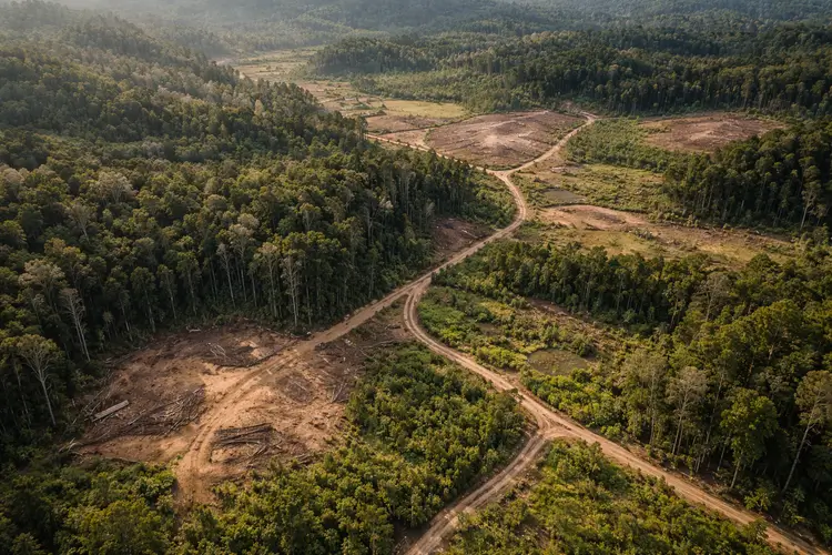
A difference between two images is not the same thing as a real change on the ground. In geospatial work, the model must separate meaningful land transitions from confounding factors such as seasonal vegetation cycles, cloud shadows, atmospheric variation, illumination differences, sensor noise, and geometric misregistration between acquisitions.

This is why change detection is a genuinely interdisciplinary problem. A model can be mathematically elegant and still perform poorly if the training data mixes winter and summer scenes carelessly, if cloud masking is inconsistent, or if the “before” and “after” images are slightly misaligned. Environmental context is part of the modeling problem, not something that can be ignored until deployment.

In many projects, the actual signal of interest is also sparse. Most pixels in a scene remain unchanged, while only a small fraction reflect meaningful change. That creates class imbalance, which means a model can achieve high accuracy by predicting “unchanged” almost everywhere and still fail at the task users care about.

That is why evaluation in this domain usually emphasizes metrics such as precision, recall, F1, and intersection-over-union rather than raw accuracy. A flood monitoring workflow and an urban expansion workflow may tolerate different error patterns, so the cost of false positives and false negatives has to be interpreted in the domain context.

Core theory: what the model is actually learning

At the simplest level, paired-image change detection can be written as:

$$\hat{y} = f_\theta(x^{(t_1)}, x^{(t_2)})$$

Here, $x^{(t_1)}$ and $x^{(t_2)}$ are co-registered images from two dates, and $\hat{y}$ is the predicted pixel-wise change map. In the binary case, each pixel is predicted as changed or unchanged. In a semantic case, the output can represent a transition class such as vegetation-to-built-up or water-to-bare-soil.

That semantic distinction matters in environmental work. A binary mask is useful for alerting and triage, but a semantic transition map is much more useful when planners, ecologists, or risk analysts need to know what changed and what the consequences may be. A new road through vegetation means something very different from seasonal wetness that turns bare ground into shallow surface water.

A common training objective combines cross-entropy with Dice loss:

$$\mathcal{L} = \lambda_{ce}\mathcal{L}_{ce} + \lambda_{dice}\mathcal{L}_{dice}$$

where the Dice term is:

$$\mathcal{L}_{dice} = 1 - \frac{2\sum_i p_i y_i + \epsilon}{\sum_i p_i + \sum_i y_i + \epsilon}$$

The reason this combination is so common is practical. Cross-entropy gives stable per-pixel supervision, while Dice helps when the positive class is sparse. In land cover change detection, the changed pixels are often a small minority, so Dice helps prevent the model from ignoring them.

For evaluation, one of the most useful metrics is IoU:

$$\text{IoU} = \frac{TP}{TP + FP + FN}$$

This is often more meaningful than accuracy because it focuses directly on how well the predicted change region overlaps the true change region. If your model is supposed to find new built-up areas, erosion fronts, or burned regions, overlap quality matters more than getting the easy, unchanged pixels right.

Why U‑Net remains a powerful baseline

U‑Net is still one of the strongest first choices for change detection because its inductive bias fits the geometry of the task. Convolution assumes local structure, translation consistency, and spatial smoothness. Those assumptions are often exactly right for roads, building edges, field boundaries, riverbanks, and forest fragments.

The encoder compresses the image into increasingly abstract features, while the decoder reconstructs spatial detail. The skip connections pass fine-grained information from the encoder to the decoder, which helps preserve boundary precision. That makes U‑Net especially strong when you care about the exact shape of the change region rather than only its approximate location.

This matters a lot in environmental analysis. A blurred urban footprint or a poorly localized riverbank change can make downstream measurement unreliable. In planning, hydrology, or land management, pixel geometry is not cosmetic. It affects area estimates, boundary calculations, and spatial overlays with administrative or ecological zones.

U‑Net also tends to be easier to train from scratch than many transformer-based alternatives. When labels are limited, compute is modest, and you need a dependable baseline quickly, this simplicity becomes a real advantage. Many teams still ship U‑Net-style systems not because they are outdated, but because they are efficient, robust, and operationally sensible.

Why transformers are attractive for geospatial change detection

Transformers replace fixed local filters with learned attention between tokens. In simplified form, self-attention can be written as:

$$\text{Attention}(Q, K, V) = \text{softmax}\left(\frac{QK^\top}{\sqrt{d_k}}\right)V$$

This allows each patch of the image to weigh information from other patches, including distant ones. In land cover change detectionthisat can be useful when a local patch is ambiguous, but its meaning becomes clearer in the context of a broader scene.

That broader context matters in many environmental settings. A small impervious patch might mean nothing in isolation, but may look different when surrounded by expanding road networks and new development. A disturbed patch in a forest may mean little on its own, but it may become more interpretable when seen as part of a larger clearing pattern.

This is why transformer-based models have gained attention in remote sensing. They are often better at modeling long-range relationships, broader spatial context, and more global scene structure. When transfer learning is available, they can also benefit from pretrained representations that improve generalization across diverse landscapes.

Still, plain ViT is not usually the best direct choice for dense segmentation. Dense prediction benefits from multiscale representations, which is why hierarchical transformer backbones such as SegFormer are often more practical. These models preserve multiscale features and pair them with lightweight decoders, making them better suited to land cover mapping and change detection than a plain classification transformer.

U‑Net vs vision transformers: the real comparison

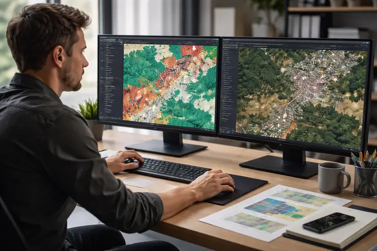
The real question is not “old CNN versus modern transformer.” The more useful framing is “strong local prior versus broader global context.” U‑Net hard-codes useful assumptions about locality and edges. Transformers relax those assumptions and let the model learn more flexible spatial relationships, often at a higher computational cost.

If your dataset is small, your labels are expensive, and your target objects depend on crisp boundaries, the U‑Net is often the better first model. It usually converges faster, is easier to debug, and makes fewer demands on hardware. That makes it especially attractive for NGOs, public-sector teams, smaller climate-tech groups, and independent geospatial researchers.

If your data spans many regions, land cover regimes, or settlement patterns, transformer backbones become more attractive. Their ability to model broader context and benefit from pretraining can help when you need cross-region generalization. This is especially relevant in large monitoring programs where the same pipeline must work across heterogeneous landscapes.

In practice, many strong systems are now hybrids. They combine convolutional feature extraction with transformer-style context modeling, or use transformer encoders with lightweight decoders. That trend reflects a deeper truth: geospatial ML rarely rewards purity. The best model is often the one that balances spatial precision, transferability, memory use, and operational cost.

Hands-on implementation in PyTorch

A fair comparison between U‑Net and a transformer should keep the data pipeline fixed and change only the backbone. That means the same input channels, the same crop size, the same augmentations, the same optimizer family, and the same evaluation protocol. Otherwise, you are not measuring architecture differences so much as pipeline differences.

The example below assumes paired four-band imagery in [R, G, B, NIR] order and a binary change mask. It also adds a simple engineered feature: delta NDVI. This is a useful example of how domain knowledge improves modeling. Remote sensing is not ordinary RGB photography, so incorporating vegetation-sensitive features can help the model separate real ecological change from ordinary image variation.

 from pathlib import Path
import numpy as np
import rasterio
import torch
from PIL import Image
from torch.utils.data import Dataset, DataLoader
from torchvision.transforms import v2 as T

EPS = 1e-6

def compute_ndvi(img: torch.Tensor) -> torch.Tensor:
    # img shape: [4, H, W] with [R, G, B, NIR]
    red = img[0]
    nir = img[3]
    return (nir - red) / (nir + red + EPS)

class PairedChangeDataset(Dataset):
    """
    root/
      sample_000/
        t1.tif
        t2.tif
        mask.png
    """

    def __init__(self, root: str, train: bool = True, crop_size: int = 256):
        self.sample_dirs = sorted([p for p in Path(root).iterdir() if p.is_dir()])
        self.transforms = None
        if train:
            self.transforms = T.Compose([
                T.RandomCrop((crop_size, crop_size)),
                T.RandomHorizontalFlip(p=0.5),
                T.RandomVerticalFlip(p=0.5),
            ])

    def __len__(self):
        return len(self.sample_dirs)

    def _read_tif(self, path: Path) -> torch.Tensor:
        with rasterio.open(path) as src:
            arr = src.read([1, 2, 3, 4]).astype("float32")
        # Example scaling for reflectance stored in 0..10000
        return torch.from_numpy(arr).clamp(0, 10000) / 10000.0

    def __getitem__(self, idx):
        d = self.sample_dirs[idx]
        t1 = self._read_tif(d / "t1.tif")
        t2 = self._read_tif(d / "t2.tif")

        mask = torch.from_numpy(
            (np.array(Image.open(d / "mask.png")) > 0).astype("int64")
        )

        delta_ndvi = (compute_ndvi(t2) - compute_ndvi(t1)).unsqueeze(0)

        # Final tensor: t1 bands + t2 bands + delta NDVI
        x = torch.cat([t1, t2, delta_ndvi], dim=0)  # [9, H, W]
        y = mask

        if self.transforms is not None:
            x, y = self.transforms(x, y)

        return x, y

The most important design choice here is not the syntax. It is the representation. By concatenating both dates plus a spectral-difference feature, you give either model a chance to learn both raw appearance change and a domain-relevant vegetation cue. That makes the comparison more realistic for environmental work than pretending every problem is just RGB computer vision with a different filename extension.

Next comes the model definition. The U‑Net below is intentionally conventional so it can serve as a clean baseline. The transformer baseline uses SegFormer rather than a plain ViT because dense segmentation usually benefits from the multiscale hierarchy and lightweight decoder that SegFormer provides.

import torch
import torch.nn as nn
import torch.nn.functional as F
from transformers import SegformerForSemanticSegmentation

class DoubleConv(nn.Module):
    def __init__(self, in_ch, out_ch):
        super().__init__()
        self.block = nn.Sequential(
            nn.Conv2d(in_ch, out_ch, 3, padding=1, bias=False),
            nn.BatchNorm2d(out_ch),
            nn.ReLU(inplace=True),
            nn.Conv2d(out_ch, out_ch, 3, padding=1, bias=False),
            nn.BatchNorm2d(out_ch),
            nn.ReLU(inplace=True),
        )

    def forward(self, x):
        return self.block(x)

class UNetChangeNet(nn.Module):
    def __init__(self, in_channels=9, num_classes=2, widths=(32, 64, 128, 256)):
        super().__init__()
        c1, c2, c3, c4 = widths
        self.enc1 = DoubleConv(in_channels, c1)
        self.enc2 = DoubleConv(c1, c2)
        self.enc3 = DoubleConv(c2, c3)
        self.enc4 = DoubleConv(c3, c4)
        self.pool = nn.MaxPool2d(2)
        self.bottleneck = DoubleConv(c4, c4 * 2)

        self.up4 = nn.ConvTranspose2d(c4 * 2, c4, 2, 2)
        self.dec4 = DoubleConv(c4 + c4, c4)
        self.up3 = nn.ConvTranspose2d(c4, c3, 2, 2)
        self.dec3 = DoubleConv(c3 + c3, c3)
        self.up2 = nn.ConvTranspose2d(c3, c2, 2, 2)
        self.dec2 = DoubleConv(c2 + c2, c2)
        self.up1 = nn.ConvTranspose2d(c2, c1, 2, 2)
        self.dec1 = DoubleConv(c1 + c1, c1)

        self.head = nn.Conv2d(c1, num_classes, 1)

    def forward(self, x):
        s1 = self.enc1(x)
        s2 = self.enc2(self.pool(s1))
        s3 = self.enc3(self.pool(s2))
        s4 = self.enc4(self.pool(s3))
        x = self.bottleneck(self.pool(s4))

        x = self.dec4(torch.cat([self.up4(x), s4], dim=1))
        x = self.dec3(torch.cat([self.up3(x), s3], dim=1))
        x = self.dec2(torch.cat([self.up2(x), s2], dim=1))
        x = self.dec1(torch.cat([self.up1(x), s1], dim=1))
        return self.head(x)

def build_segformer_change_model(num_classes=2, in_channels=9):
    model = SegformerForSemanticSegmentation.from_pretrained(
        "nvidia/segformer-b0-finetuned-ade-512-512",
        num_labels=num_classes,
        ignore_mismatched_sizes=True,
    )

    old_proj = model.segformer.encoder.patch_embeddings[0].proj
    new_proj = nn.Conv2d(
        in_channels,
        old_proj.out_channels,
        kernel_size=old_proj.kernel_size,
        stride=old_proj.stride,
        padding=old_proj.padding,
        bias=(old_proj.bias is not None),
    )

    with torch.no_grad():
        new_proj.weight.zero_()
        keep = min(old_proj.in_channels, in_channels)
        new_proj.weight[:, :keep] = old_proj.weight[:, :keep]

        if in_channels > old_proj.in_channels:
            mean_w = old_proj.weight.mean(dim=1, keepdim=True)
            extra = in_channels - old_proj.in_channels
            new_proj.weight[:, old_proj.in_channels:] = mean_w.repeat(1, extra, 1, 1)

        if old_proj.bias is not None:
            new_proj.bias.copy_(old_proj.bias)

    model.segformer.encoder.patch_embeddings[0].proj = new_proj
    return model

def forward_logits(model, x):
    out = model(x)
    logits = out.logits if hasattr(out, "logits") else out
    if logits.shape[-2:] != x.shape[-2:]:
        logits = F.interpolate(logits, size=x.shape[-2:], mode="bilinear", align_corners=False)
    return logits

The transformer initialization is worth pausing on. In remote sensing, you often need more than three input channels. Replacing the first projection layer lets you adapt an RGB-pretrained model to multispectral or paired-date data without discarding all the pretrained weights. That is one of the main reasons transformers become attractive in practice: they can import useful large-scale visual priors even when the downstream geospatial task is relatively small.

Training should reflect the class imbalance typical of change detection. Precision, recall, F1, and IoU are usually more informative than raw accuracy because unchanged pixels dominate the map. A model that predicts “unchanged” almost everywhere can look fine under accuracy and still be useless for actual environmental monitoring. Remote-sensing reviews consistently emphasize metrics derived from TP, FP, TN, and FN for exactly this reason.

import time
from torch.optim import AdamW

def dice_loss(logits, targets, eps=1e-6):
    probs = logits.softmax(dim=1)[:, 1]
    targets = targets.float()
    inter = (probs * targets).sum(dim=(1, 2))
    union = probs.sum(dim=(1, 2)) + targets.sum(dim=(1, 2))
    return 1.0 - ((2 * inter + eps) / (union + eps)).mean()

@torch.no_grad()
def evaluate(model, loader, device):
    model.eval()
    confmat = torch.zeros(2, 2, dtype=torch.float64, device=device)

    for x, y in loader:
        x = x.to(device)
        y = y.to(device)
        preds = forward_logits(model, x).argmax(dim=1)
        hist = torch.bincount((y * 2 + preds).view(-1), minlength=4).reshape(2, 2)
        confmat += hist

    tn, fp, fn, tp = confmat[0, 0], confmat[0, 1], confmat[1, 0], confmat[1, 1]
    precision = tp / (tp + fp + 1e-6)
    recall = tp / (tp + fn + 1e-6)
    f1 = 2 * precision * recall / (precision + recall + 1e-6)
    iou = tp / (tp + fp + fn + 1e-6)

    return {
        "precision": float(precision),
        "recall": float(recall),
        "f1": float(f1),
        "iou": float(iou),
    }

@torch.no_grad()
def latency_ms(model, sample, device="cuda", warmup=10, runs=50):
    model.eval().to(device)
    sample = sample.to(device)

    for _ in range(warmup):
        _ = forward_logits(model, sample)

    if device.startswith("cuda"):
        torch.cuda.synchronize()

    t0 = time.perf_counter()
    for _ in range(runs):
        _ = forward_logits(model, sample)

    if device.startswith("cuda"):
        torch.cuda.synchronize()

    return 1000.0 * (time.perf_counter() - t0) / runs

device = "cuda" if torch.cuda.is_available() else "cpu"

train_ds = PairedChangeDataset("data/train", train=True)
val_ds = PairedChangeDataset("data/val", train=False)

train_loader = DataLoader(train_ds, batch_size=8, shuffle=True, num_workers=4, pin_memory=True)
val_loader = DataLoader(val_ds, batch_size=8, shuffle=False, num_workers=4, pin_memory=True)

model = UNetChangeNet(in_channels=9, num_classes=2).to(device)
# model = build_segformer_change_model(num_classes=2, in_channels=9).to(device)

optimizer = AdamW(model.parameters(), lr=3e-4, weight_decay=1e-4)
ce_loss = nn.CrossEntropyLoss(weight=torch.tensor([0.2, 0.8], device=device))

for epoch in range(20):
    model.train()
    for x, y in train_loader:
        x = x.to(device)
        y = y.to(device)

        logits = forward_logits(model, x)
        loss = ce_loss(logits, y) + 0.5 * dice_loss(logits, y)

        optimizer.zero_grad(set_to_none=True)
        loss.backward()
        optimizer.step()

    metrics = evaluate(model, val_loader, device)
    print(f"epoch={epoch:02d} f1={metrics['f1']:.4f} iou={metrics['iou']:.4f}")

x0, _ = next(iter(val_loader))
print(f"latency_ms={latency_ms(model, x0[:1], device=device):.2f}")

A sensible experimental pattern is to start with U‑Net, establish a strong baseline, and then swap in SegFormer while keeping everything else fixed. If the transformer gives better F1 or IoU but significantly worse latency and memory use, that is a real trade-off you can reason about. For many environmental teams, that trade-off is more important than squeezing out a marginal benchmark gain.

The design of the input tensor is worth noting. Both dates are provided directly, but the model also gets delta NDVI as an explicit vegetation-change cue. This is a good example of interdisciplinary feature design. Even in deep learning, remote sensing often benefits from spectral knowledge rather than relying entirely on the model to rediscover known physical relationships.

The U‑Net baseline is deliberately plain. That is a strength, not a weakness, because it helps you establish a credible baseline before moving to more complex models. The transformer option uses SegFormer because hierarchical transformer encoders tend to make more sense for dense segmentation than a plain ViT classifier backbone.

If you run both models under the same conditions, you often see a recognizable pattern. U‑Net converges faster and may produce sharper boundaries, especially on smaller datasets. The transformer baseline may become more attractive when pretrained weights and broader scene context improve generalization, but that advantage must be measured rather than assumed.

How to evaluate the models in a way that matters

In change detection, accuracy can be misleading because unchanged pixels dominate. That is why precision, recall, F1, and IoU are usually better choices. These metrics tell you whether the model is missing important changes, over-predicting them, or balancing the two reasonably well.

The right metric emphasis depends on the domain. In illegal land clearing or flood extent mapping, missing a real change may be more costly than reviewing a few extra false positives. In urban growth screening over huge areas, false positives may become expensive because they create too much analyst review work.

Latency matters too. In a notebook experiment, it is easy to focus only on F1. In production, you should also ask how many milliseconds a tile takes, how much VRAM the model uses, how large a batch it can handle, and how expensive it becomes when scaled to a whole region or country.

This is often where U‑Net retains an operational advantage. A model that is slightly worse on a benchmark but much cheaper to run may be the better system if it allows more frequent updates, wider coverage, or more robust deployment. In environmental AI, the best model is often the one that fits both the science and the infrastructure.

Systems and production considerations at scale

Most land cover change detection systems run as batch pipelines rather than interactive APIs. The Earth observation process itself is periodic, so the inference workflow usually follows the cadence of incoming imagery. Teams may run weekly, monthly, seasonal, or event-driven jobs depending on whether they are monitoring routine land transitions or responding to disasters.

That means data engineering is central. You need repeatable ingestion, cloud masking, reprojection, band alignment, tiling, metadata tracking, and storage formats that work efficiently in distributed environments. Model quality will suffer if any of those steps are inconsistent, and debugging becomes difficult when the data lineage is unclear.

This is one reason why standards such as STAC and formats such as Cloud Optimized GeoTIFF are so useful in practice. They help teams organize large spatiotemporal collections and read only the spatial chunks they need. In many real systems, those engineering choices improve throughput and reproducibility as much as switching from one backbone to another.

Infrastructure choices also affect architecture choices. If the pipeline must run cheaply on modest GPUs or even CPUs, the U‑Net becomes attractive because it is simpler and more predictable. If the team has access to stronger infrastructure and the monitoring scope spans highly diverse regions, a transformer-based model may justify its cost through better transfer performance.

Monitoring is also domain-specific. In addition to model outputs, you should track cloud contamination, acquisition time gaps, band availability, registration quality, tile failure counts, and geographic drift. A sudden jump in false positives might reflect monsoon-season imagery, poor alignment, or sensor artifacts rather than a “bad model” in the abstract.

Risks, ethics, safety, and governance

The first major risk is representativeness. Many public benchmarks are geographically narrow or task-specific. A model trained on building changes in one region may not generalize to peri-urban expansion in another region, let alone to wetland transitions, wildfire scars, or mountainous terrain with strong seasonal effects.

The second risk is over-interpretation. Domain experts may be tempted to treat a change map as ground truth when it is only a model output based on imperfect imagery and labels. In environmental and public-sector settings, this can lead to poor downstream decisions if uncertainty is not communicated clearly.

There are also privacy and governance questions. Public satellite imagery is not automatically personal data, but derived products can still become sensitive when linked to parcels, households, protected areas, operational routines, or enforcement processes. This is especially true when outputs are combined with administrative or proprietary datasets.

A sensible governance approach includes documented data lineage, clear access controls, geographic holdout evaluation, uncertainty reporting, and human review for high-impact decisions. In other words, a responsible change detection system is not just a model with a good score. It is a process that makes its assumptions and limitations visible.

Security matters as well. Geospatial ML pipelines often combine cloud storage, ETL jobs, notebooks, model training infrastructure, and downstream dashboards. That creates many opportunities for weak access control, configuration drift, or accidental leakage. Good ML engineering in this domain includes secure storage, role-based permissions, reproducible builds, and logging that allows teams to audit how a map was produced.

Case study: peri-urban expansion and vegetation loss

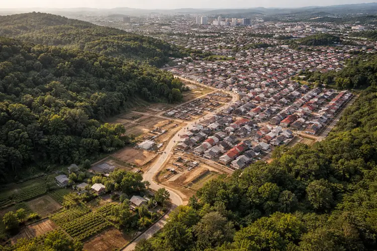
Imagine a regional planning team wants to monitor how a growing city is expanding into vegetated land at its edges. The technical problem is binary or semantic change detection. The domain problem is broader: identify where impervious surface growth may increase runoff, reduce green cover, and intensify local heat stress.

A realistic data setup might use two seasonal composites from Sentinel‑2, plus a set of manually reviewed training masks. The main challenges would include cloud contamination, seasonal vegetation variation, and imperfect alignment between acquisitions. Those challenges are ordinary in remote sensing, which is exactly why the ML pipeline has to be designed with domain awareness.

For a first production-ready baseline, U‑Net is often the best choice. It is easier to train, more forgiving with limited labels, and well-suited to detecting the boundaries of roads, parcels, and newly built surfaces. If the project later expands to multiple cities across different countries and climates, a transformer-based model becomes more attractive because broader context and pretrained features may improve cross-region consistency.

The output should not stop at a pretty mask. The planning team will usually need summaries by district or watershed, uncertainty flags around ambiguous regions, and a review queue for the highest-impact changes. This is a good reminder that the ML model is part of an environmental decision system, not the whole system.

Skills Mapping and Learning Path

This topic is especially valuable in a bootcamp-style learning path because it develops multiple skill layers at once. On the programming side, you build practical experience with Python data pipelines, raster data handling, custom datasets, augmentation strategies, and structured experimentation workflows.

On the machine learning side, you deepen your understanding of segmentation problems. This includes working with loss functions, handling class imbalance, comparing architectures like U-Net and transformer-based models, and designing evaluation metrics that reflect real-world performance.

From a systems perspective, you move beyond isolated notebook experiments into production thinking. You learn tiled inference, cloud-friendly geospatial data formats, job orchestration, and how to benchmark models across different hardware environments.

The domain layer is equally critical. Environmental data introduces challenges such as seasonality, cloud cover, spatial misalignment, and spectral variability. You also learn how analysts interpret outputs in planning, climate monitoring, and land management contexts.

A strong progression starts with datasets such as OSCD or LEVIR-CD. Begin by building a reliable U-Net baseline, then introduce a transformer-based model like SegFormer under identical training conditions to ensure a fair comparison.

Once the baseline is stable, incorporate domain-aware improvements. Add preprocessing steps such as cloud masking, seasonal compositing, and spectral indices like NDVI. This bridges the gap between generic computer vision and real-world geospatial modeling.

The next stage is operational. Package your workflow into a reproducible pipeline, benchmark cost and latency, and test generalization across geographically distinct regions. This is where a project becomes production-ready rather than purely academic.

If you want structured guidance to build these skills step by step, explore the Data Science & AI Bootcamp. It is designed to help you move from fundamentals to production-level machine learning with real-world projects.

You can also accelerate your learning through hands-on practice in the Free Tech Workshops, where you work on applied coding and AI use cases in a guided environment.

Conclusion

U-Net remains one of the strongest baselines for land cover change detection because it aligns well with the spatial structure of geospatial data. It is efficient, stable, and particularly effective when working with limited labeled datasets and tasks that require precise boundaries.

Vision transformers and hierarchical transformer models become more compelling when broader spatial context, pretraining, and cross-region generalization become important. However, they are not a free upgrade and introduce trade-offs in memory usage, latency, and system complexity.

The most useful way to approach this comparison is not as a trend debate. It is a design decision based on inductive bias, infrastructure constraints, and the actual needs of the environmental application.

A model that performs slightly better in isolation may not be the best choice if it is too slow, too costly, or difficult to deploy at scale. In real-world monitoring systems, reliability and efficiency often matter as much as raw accuracy.

If you want to go deeper, don’t just compare architectures in theory. Run controlled experiments on real paired-image datasets, evaluate both segmentation quality and operational cost, and interpret the results within a real environmental use case.

To continue building practical, job-ready skills in machine learning and applied AI, you can also explore the full learning path and career support options at Code Labs Academy, including personalized guidance through the Career Services Center.